
Funnel Plot Generator for meta-analysis
Upload one row per study and get a publication-ready funnel plot: effect size against standard error, pseudo 95% confidence limits around the pooled estimate and Egger’s test for asymmetry. Add contour shading or trim-and-fill when you need them. No R or Stata required.
Free account · daily credits included · no credit card
Example result · reference figure drawn from this sample data
Funnel plot examples
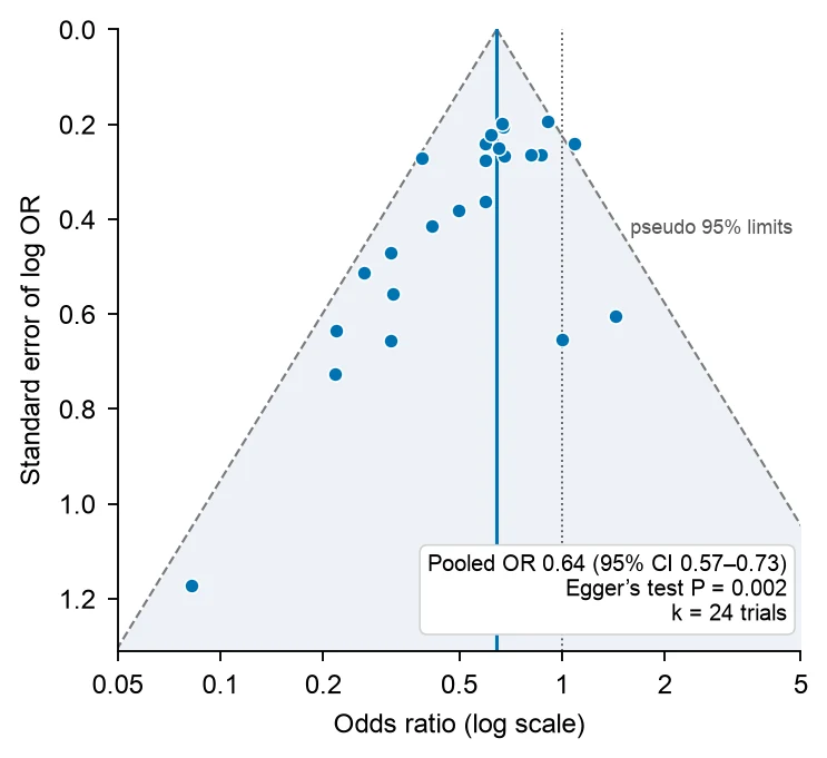
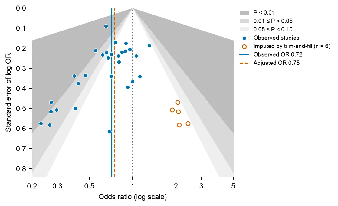
These are reference figures drawn from the sample datasets above (simulated trials with small-study effects built in), not FigCanvas outputs; the prompts are what you would ask FigCanvas for. In the 24-trial example the fixed-effect pooled OR is 0.64 (95% CI 0.57–0.73) and Egger’s test gives P = 0.002. In the 30-study example (Egger’s P = 0.022), trim-and-fill imputes 6 studies on the right of the funnel and moves the pooled OR from 0.72 to 0.75.
What a funnel plot shows
A funnel plot is a scatter plot of the studies in a meta-analysis: each study’s effect estimate on the x-axis against its standard error, a measure of its precision, on the y-axis. It is the standard visual check for small-study effects and possible publication bias in a systematic review, and it usually sits next to the forest plot of the same meta-analysis.
How to read a funnel plot
The y-axis is inverted, so large, precise studies sit at the top and small studies spread out at the bottom. Ratio measures such as odds ratios and risk ratios are plotted on a log scale. The vertical line is the pooled estimate, and the diagonal lines are pseudo 95% confidence limits: pooled estimate ± 1.96 × standard error.
Without bias or heterogeneity, about 95% of the studies fall inside those limits and scatter evenly on both sides of the pooled line, giving the shape of an inverted funnel. A gap in one bottom corner, usually small studies with null or unfavourable results, makes the plot asymmetric.
Asymmetry is not proof of publication bias
Asymmetry means that small studies report different effects from large ones, which is why it is called a small-study effect. Publication bias is one cause. Others listed by Sterne et al. (BMJ 2011) are poorer methodological quality in small trials, true heterogeneity (small trials often enrol higher-risk patients or deliver a more intensive intervention), artefacts of the effect measure, and chance.
Report asymmetry as a small-study effect and discuss the possible causes. A contour-enhanced funnel plot (below) helps tell them apart.
Egger’s test and the 10-study rule
Egger’s regression test (Egger et al., BMJ 1997) regresses each study’s standardized effect (effect ÷ standard error) on its precision (1 ÷ standard error). With no asymmetry the intercept is close to zero. Egger used P < 0.10 rather than 0.05 because the test has low power.
Sterne et al. (BMJ 2011) and the Cochrane Handbook advise using funnel plot asymmetry tests only when a meta-analysis has at least 10 studies, because with fewer the tests cannot tell chance from real asymmetry. For odds ratios, Egger’s test can give false positives, and the Harbord (2006) or Peters (2006) tests are often preferred.
Contour-enhanced funnel plots and trim-and-fill
A contour-enhanced funnel plot (Peters et al., Journal of Clinical Epidemiology 2008) shades the regions where a study would reach P < 0.01, 0.01–0.05 and 0.05–0.10 against the null. If the missing studies would fall in the non-significant white area, publication bias becomes more plausible. If the gap is in an area of significance, other causes are more likely.
Trim-and-fill (Duval and Tweedie, Biometrics 2000) estimates how many studies are missing from the sparse side. It removes the most extreme studies from the crowded side, re-estimates the centre, and adds mirror images of the removed studies. Treat the adjusted estimate as a sensitivity analysis, not a corrected result: it assumes that all the asymmetry comes from publication bias.
How to lay out data for a funnel plot
Use one row per study. FigCanvas detects the columns by name and content, and you can confirm the mapping before plotting. The same file can drive the forest plot of the meta-analysis.
- study
- Study label, for example first author and year. Used to label outliers and in the table of results.
- effect
- The effect estimate: odds ratio, risk ratio, hazard ratio, mean difference or standardized mean difference. Ratios can be given as is or on the log scale.
- se or CI
- The standard error of the effect, or the lower and upper 95% confidence limits. For ratios, the standard error of the log ratio is (ln upper − ln lower) ÷ 3.92.
- counts
- Optional instead of the effect: events and totals in each arm of a 2×2 table, from which the log odds ratio and its standard error are computed.
| study | odds_ratio | ci_lower | ci_upper |
|---|---|---|---|
| Trial 01 (2004) | 0.670 | 0.447 | 1.005 |
| Trial 02 (2004) | 0.598 | 0.373 | 0.959 |
| Trial 03 (2006) | 0.082 | 0.008 | 0.789 |
| Trial 04 (2008) | 0.679 | 0.402 | 1.146 |
Use the same effect measure for every study. If some studies report medians or only P values, convert them first or ask FigCanvas to help with the conversion, and say which method you used in the methods section.
How to make a funnel plot with FigCanvas
Go from study effect sizes to a publication-ready funnel plot in four steps.
Upload the study data
Upload a CSV or Excel file with one row per study (effects with standard errors, ratios with confidence intervals, or 2×2 counts), or load one of the sample datasets.
Confirm columns and options
FigCanvas identifies the effect, its standard error or confidence interval and the effect scale, then proposes the plot: pooled estimate, pseudo 95% limits and Egger’s test.
Generate the figure
The inverse-variance pooled estimate and Egger’s regression are computed from your data in Python with statsmodels, and the funnel is drawn with journal-style defaults and colorblind-safe colors.
Refine and export
Ask for contour shading, trim-and-fill, random effects, study labels or a different axis range in plain language, then export SVG, PDF or PNG for the manuscript.
Why researchers make their figures with FigCanvas
Statistics computed, not drawn
The pooled estimate, the confidence limits and the Egger’s test P value come from Python code run on your data. The figure is reproducible, and you can read the code.
Contours and trim-and-fill on request
Add significance contours, imputed studies and the adjusted estimate to the same figure without a separate package for each.
No R or Stata licence
Skip metafor syntax and Stata menus. Upload the extraction sheet from your systematic review and get the figure in about a minute.
Editable vector export
Export SVG or PDF and adjust fonts, labels or panel layout in Illustrator or Inkscape to match the journal’s figure guidelines.
Funnel plot FAQs
Yes. Upload a CSV or Excel file with one row per study, its effect size and standard error (or 95% CI), and the FigCanvas funnel plot generator draws the funnel with the pooled effect line and pseudo 95% confidence limits and runs Egger’s test. You can sign up for free and make funnel plots with the free daily credits.
Upload the table you already have and say what you need, for example “funnel plot of log odds ratio against standard error, Egger’s test and trim-and-fill”. FigCanvas writes and runs Python code on your data, pooling the studies and running Egger’s regression with statsmodels, so the numbers are computed, not drawn. In R the same takes funnel(), regtest() and trimfill() from metafor.
One row per study with an effect size and its standard error. For odds ratios, risk ratios or hazard ratios, use the log scale, or give the 95% CI and FigCanvas derives the standard error as (ln upper − ln lower) ÷ 3.92. Mean differences and standardized mean differences work as they are. Raw 2×2 counts (events and totals in each arm) can be converted to log odds ratios for you.
Yes. Egger’s test (BMJ 1997) regresses each study’s effect ÷ SE on its precision; an intercept away from zero means asymmetry, and P < 0.10 is often used because the test has low power. Trim-and-fill (Duval and Tweedie, Biometrics 2000) imputes the studies missing from the sparse side and gives an adjusted estimate; report it as a sensitivity analysis. In the examples above, Egger’s test gives P = 0.002 for 24 trials, and trim-and-fill imputes 6 of 30 studies and moves the pooled odds ratio from 0.72 to 0.75.
Yes; ask for shaded regions at P < 0.10, 0.05 and 0.01. If the missing studies would fall in the non-significant region, publication bias is a more plausible cause of the asymmetry; if they would be significant, look for other causes such as heterogeneity or lower quality in small studies (Sterne et al., BMJ 2011).
Show the funnel plot with the pooled estimate line and pseudo 95% confidence limits, and report Egger’s intercept with its 95% CI and P value and the number of studies. If you ran trim-and-fill, give the number of imputed studies and the adjusted pooled estimate. Say that asymmetry can come from small-study effects or heterogeneity, not only publication bias.
You can draw it, but Sterne et al. (BMJ 2011) and the Cochrane Handbook advise against asymmetry tests with fewer than 10 studies, or when all studies are of similar size, because the tests have too little power. Show the plot if a reviewer asks for it, and state that Egger’s test was not run and why.
Pro and Credit Pack users export editable SVG and 300 DPI PDF, so labels and fonts can be adjusted in Illustrator or Inkscape to the journal’s guidelines; free exports are watermarked PNG. If the journal asks for TIFF, export a PNG and convert it with the free FigCanvas PNG to TIFF converter.
In R, funnel() and trimfill() in metafor, or funnel() in meta; in Stata 16 and later, meta funnelplot and meta bias. RevMan, Cochrane’s review software, draws funnel plots for Cochrane reviews, and JASP is free and point-and-click. Comprehensive Meta-Analysis is paid. FigCanvas makes a funnel plot from a CSV of effect sizes and standard errors, with Egger’s test and trim-and-fill, without code.
Only by hand. Compute the log effect and its standard error ((ln upper − ln lower) ÷ 3.92 from a 95% CI), make a scatter chart of the log effect against the standard error, reverse the y-axis, and add two lines for pooled ± 1.96 × SE. Egger’s test needs a separate regression. To skip that, upload the same table to the FigCanvas funnel plot generator.
Make a funnel plot from your meta-analysis data
Upload effect sizes and standard errors, get the funnel plot with pseudo 95% limits and Egger’s test, then export it for your systematic review.
More AI tools for scientific figures
View all tools →
Forest Plot Generator
Forest plots for meta-analysis, systematic reviews and regression results with confidence intervals.
Open tool →
PRISMA Flow Diagram Generator
PRISMA 2020 flow diagrams for systematic reviews and meta-analyses, drawn from your screening counts.
Open tool →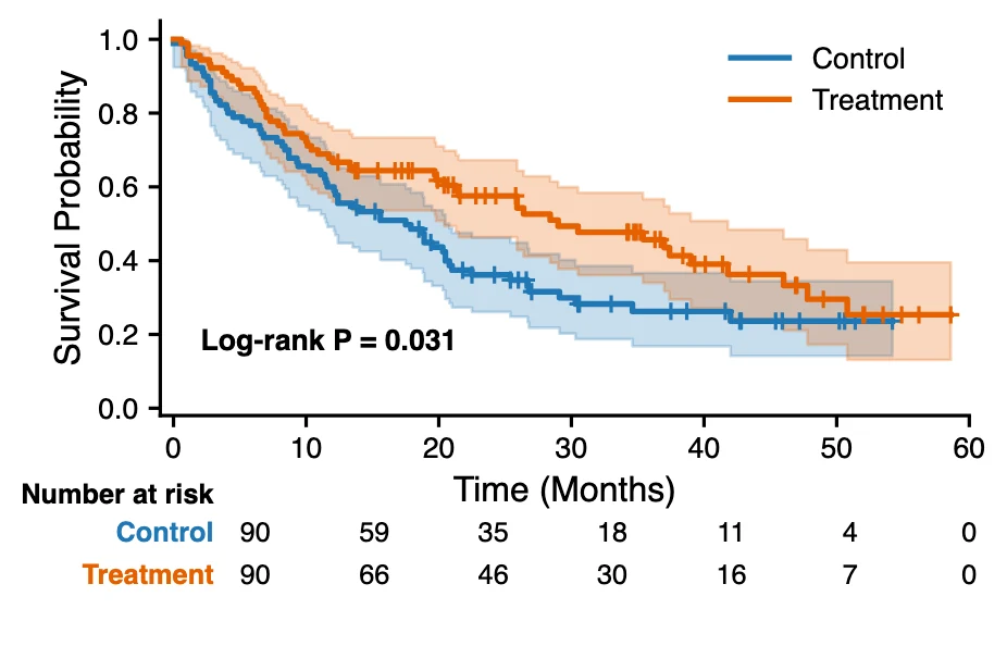
Kaplan-Meier Curve Generator
Kaplan-Meier survival curves with censoring marks, log-rank test and a number-at-risk table from time-to-event data.
Open tool →