
Manhattan Plot Generator for GWAS results
Upload GWAS summary statistics and get a publication-ready Manhattan plot with the genome-wide significance line at 5×10⁻⁸, the suggestive line at 1×10⁻⁵ and labeled lead SNPs, plus a QQ plot with the genomic inflation factor λ. No R or qqman required.
Free account · daily credits included · no credit card
Example result · reference figure drawn from this sample data
Manhattan plot examples
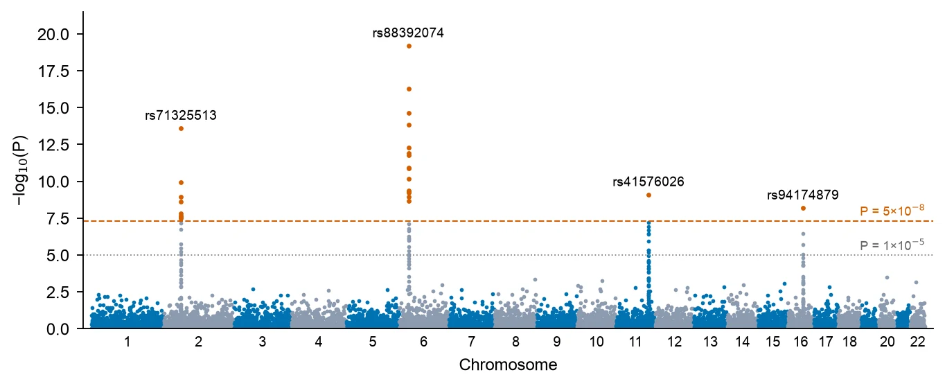
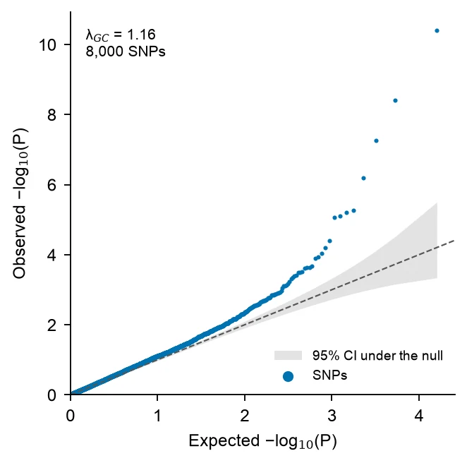
These are reference figures drawn from the sample datasets above (simulated GWAS of the 22 autosomes, thinned to 9,000 and 8,000 SNPs), not FigCanvas outputs; the prompts are what you would ask FigCanvas for. In the Manhattan example 27 SNPs in 4 loci pass P < 5×10⁻⁸, the strongest on chromosome 6 at P = 6.3×10⁻²⁰, and λ is 1.03. The QQ example comes from a second simulated GWAS with λ = 1.16, the early lift-off from the diagonal that points to population stratification.
What a Manhattan plot shows
A Manhattan plot shows the result of a genome-wide association study (GWAS) in one figure: every tested variant is a point, placed by its position along the genome on the x-axis and by −log10 of its P value on the y-axis. Strong associations rise as towers above a dense band of null results, like skyscrapers on a skyline, which gives the plot its name.
How to read a Manhattan plot
Chromosomes run left to right in alternating colors, and positions within each chromosome are in base pairs. The higher a point, the smaller its P value: −log10(P) = 7.3 corresponds to P = 5×10⁻⁸, and 20 to P = 10⁻²⁰.
A real association looks like a tower, not a single point, because neighbouring variants in linkage disequilibrium with the causal variant carry part of the signal. An isolated point high above an empty region is more often a genotyping or imputation artefact and should be checked before it is reported.
Genome-wide and suggestive significance lines
The genome-wide significance threshold of P < 5×10⁻⁸ is a Bonferroni correction of 0.05 for about one million independent common-variant tests in European-ancestry genomes (Pe’er et al., Genetic Epidemiology 2008). It is drawn as a horizontal line at −log10(P) = 7.3. Studies of rare variants from whole-genome sequencing sometimes use stricter thresholds, such as the 5×10⁻⁹ proposed by Pulit et al. (2017).
The suggestive line at P < 1×10⁻⁵ (−log10(P) = 5) marks signals worth following up in a replication sample. It is a convention, not a significance claim: with a million independent tests, about 10 variants pass it by chance alone.
The QQ plot and genomic inflation λ
A quantile-quantile (QQ) plot sorts the observed −log10(P) values and plots them against the values expected if no variant were associated. Under the null, the points follow the diagonal. A few points lifting off at the top right are the true associations. A whole curve that leaves the diagonal early points to systematic inflation.
The genomic inflation factor λ (Devlin and Roeder, Biometrics 1999) is the median of the observed association chi-square statistics divided by 0.4549, the median of a chi-square distribution with 1 degree of freedom. Values near 1.0 are expected. λ above about 1.05–1.10 calls for checking population stratification, cryptic relatedness or batch effects. Highly polygenic traits in very large samples also inflate λ without any confounding, and the LD score regression intercept (Bulik-Sullivan et al., Nature Genetics 2015) separates the two.
Counting loci and labeling lead SNPs
Report loci, not SNPs. Dozens of correlated variants can pass the threshold at one locus, so they are grouped by distance (for example within 500 kb) or by linkage disequilibrium with PLINK clumping, and each locus is represented by its lead SNP, the variant with the smallest P value.
Label the lead SNP of each locus with its rs number or the nearest gene, and highlight the variants of the locus in a contrasting color. Keep labels to the genome-wide loci: labeling every suggestive peak makes the figure unreadable.
How to lay out data for a Manhattan plot
Use one row per variant. Output from PLINK, REGENIE, SAIGE, BOLT-LMM or the GWAS Catalog usually works as is: FigCanvas detects the chromosome, position and P value columns by name and content, and you can confirm the mapping before plotting.
- chr
- Chromosome, as 1–22 or chr1–chr22. X, Y and MT can be drawn after the autosomes.
- bp
- Base-pair position on that chromosome. Use one genome build (GRCh37 or GRCh38) for the whole file.
- p
- Association P value. A −log10(P) column, such as LOG10P from REGENIE, also works.
- snp
- Optional. Variant id such as an rs number, used to label the lead SNPs.
| snp | chr | bp | p |
|---|---|---|---|
| rs12180834 | 1 | 593329 | 0.928 |
| rs20659145 | 1 | 639929 | 0.127 |
| rs61316584 | 1 | 841557 | 0.508 |
| rs54543422 | 1 | 2226710 | 0.467 |
Full summary statistics work: λ and the QQ plot need every variant, and for the Manhattan plot FigCanvas can thin the non-significant SNPs (keep everything below P = 0.01 and a random sample of the rest), which leaves the figure unchanged but keeps vector files small. The upload on this page takes files up to 10 MB, about 300,000 rows of these four columns; for a genome-wide file of millions of variants, drop the extra columns or thin it before uploading.
How to make a Manhattan plot with FigCanvas
Go from GWAS summary statistics to a publication-ready Manhattan plot in four steps.
Upload summary statistics
Upload a CSV, TSV or Excel file with chromosome, position and P value for each variant, or load one of the sample datasets.
Confirm columns and options
FigCanvas identifies the chromosome, position, P value and SNP id columns and proposes the figure: significance lines, colors, lead SNP labels and an optional QQ plot.
Generate the figure
Cumulative genome positions, −log10(P), the loci above 5×10⁻⁸ and λ are computed from your data in Python with pandas and SciPy, and the plot is drawn with journal-style defaults and colorblind-safe colors.
Refine and export
Change thresholds, colors, labels or the chromosome range by asking in plain language, add the QQ plot as a second panel, then export SVG, PDF or PNG.
Why researchers make their figures with FigCanvas
Thresholds and λ computed, not drawn
Significance lines, the loci that pass them and the genomic inflation factor come from Python code run on your data, so the figure matches your summary statistics.
Manhattan and QQ plot together
Ask for the QQ plot in the same session and get both panels with the same styling, ready for the main figure or the supplement.
No R or qqman setup
Skip installing qqman or CMplot and renaming columns to CHR, BP and P. Upload the file your GWAS software wrote and confirm the mapping.
Editable vector export
Export SVG or PDF and adjust labels, fonts or panel size in Illustrator or Inkscape to match the journal’s figure guidelines.
Manhattan plot FAQs
Yes. Upload GWAS summary statistics with chromosome, position and P value, and the FigCanvas Manhattan plot generator draws the Manhattan plot with the genome-wide (5×10⁻⁸) and suggestive (1×10⁻⁵) lines, labels the lead SNPs, and makes the QQ plot with the genomic inflation factor λ. You can sign up for free and make Manhattan and QQ plots with the free daily credits.
Upload the file and describe the plot, for example “Manhattan plot with alternating chromosome colors, lines at 5×10⁻⁸ and 1×10⁻⁵, label the top SNP per locus, plus a QQ plot”. FigCanvas writes and runs the Python code on your data, so the figure can be reproduced and changed in the same chat. In R this is manhattan() and qq() from qqman.
Yes. Files from PLINK, REGENIE, SAIGE, BOLT-LMM or the GWAS Catalog usually work without renaming columns, and FigCanvas can thin the non-significant SNPs so the plot stays light. The upload on this page takes files up to 10 MB, about 300,000 rows of chromosome, position, P value and SNP id. For larger files, keep only those four columns or thin out SNPs with P > 0.01 before uploading.
Chromosome, base-pair position and P value, plus an optional SNP id for labels. Names such as CHR, BP and P from PLINK, CHROM, GENPOS and LOG10P from REGENIE (which reports −log10 P), or chromosome, base_pair_location and p_value from the GWAS Catalog format are understood without renaming. Chromosomes X, Y and MT can be kept or dropped.
Yes. The QQ plot compares the sorted observed −log10(P) with the values expected if no variant were associated, and λ is the median association chi-square divided by 0.4549 (Devlin and Roeder, 1999). λ up to about 1.05 is usually accepted; above about 1.1, check population structure, although large studies of polygenic traits can exceed it with no confounding. The second example above has λ = 1.16.
Yes; ask for the top SNP per locus by rsID, or supply a nearest-gene column to use as labels. Say how loci are defined, for example a distance window around each lead SNP or LD clumping done beforehand in PLINK. In the example above, 27 SNPs pass 5×10⁻⁸ and form 4 loci, on chromosomes 2, 6, 11 and 16.
The number of variants and samples, the test or model and its covariates, what the two lines mark (genome-wide significance at 5×10⁻⁸ and the suggestive level at 1×10⁻⁵), the genome build, and the genomic inflation factor λ from the QQ plot. Label lead SNPs by rsID or nearest gene, and say how independent loci were defined.
Pro and Credit Pack users export editable SVG and 300 DPI PDF; free exports are watermarked PNG. With hundreds of thousands of points, ask for the point layer to be rasterized so the PDF stays small while the axes and labels stay vector. If the journal asks for TIFF, export a PNG and convert it with the free FigCanvas PNG to TIFF converter.
In R, qqman is the simplest (manhattan() and qq()), and CMplot draws circular and multi-trait versions; in Python, GWASLab or matplotlib. FUMA, a free web platform, draws Manhattan and QQ plots as part of annotating uploaded summary statistics, and LocusZoom draws regional plots of a single locus. FigCanvas makes a Manhattan plot and QQ plot from a CSV of chromosome, position and P value, with significance lines and labeled lead SNPs, without code.
Excel is impractical: a sheet holds at most 1,048,576 rows, fewer than a typical imputed GWAS, and has no genomic axis. In Python, read the file with pandas, add each chromosome’s cumulative length to the positions, compute −log10(P), and scatter by chromosome in matplotlib with axhline at 7.3 and 5; λ is np.median(scipy.stats.chi2.isf(p, 1)) / 0.4549. Without code, upload the file to the FigCanvas Manhattan plot generator.
Make a Manhattan plot from your GWAS results
Upload summary statistics, get the Manhattan plot with significance lines and labeled loci plus a QQ plot with λ, then export it for your paper.
More AI tools for scientific figures
View all tools →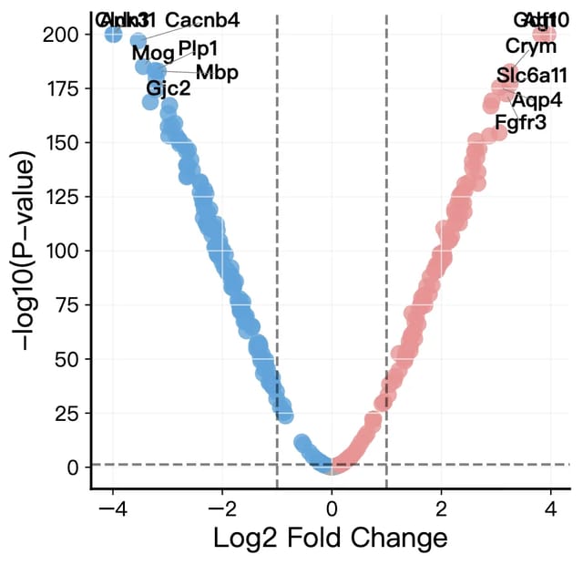
Volcano Plot Maker
Volcano plots for RNA-seq, proteomics and GWAS results with labeled genes and significance thresholds.
Open tool →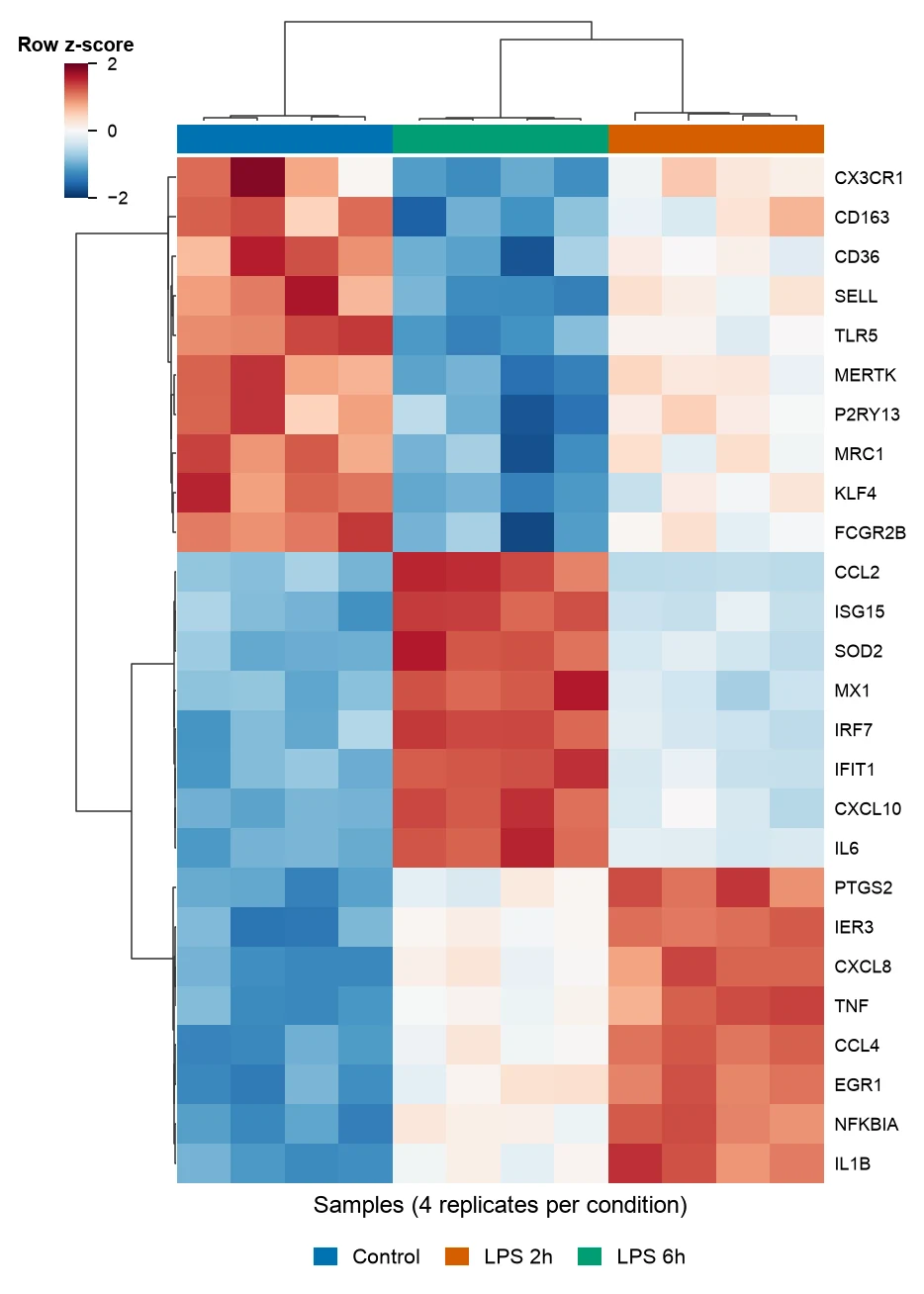
Heatmap Generator
Clustered gene expression heatmaps with z-scored rows and dendrograms, and correlation heatmaps of any numeric table.
Open tool →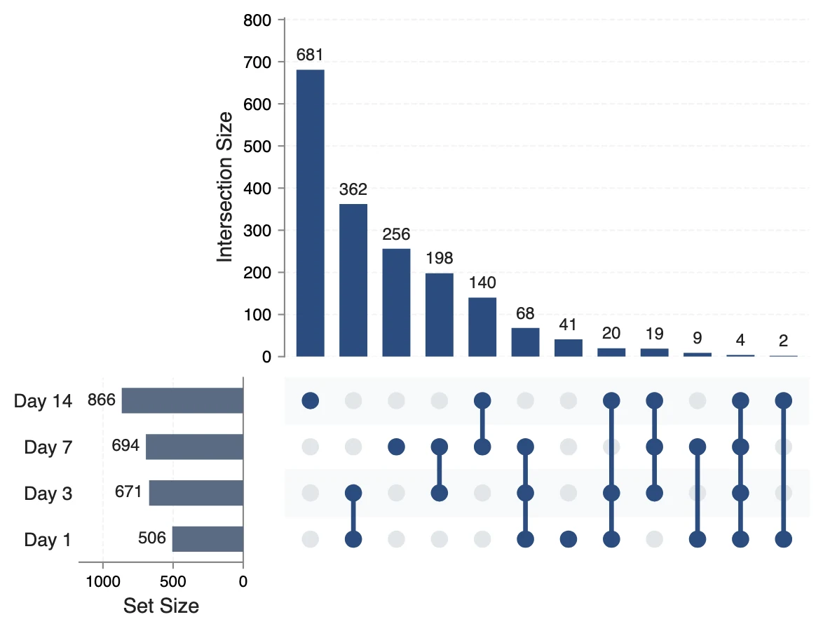
UpSet Plot Generator
UpSet plots of gene lists, variant calls or any sets, for overlaps a Venn diagram cannot show.
Open tool →