
Free AI Heatmap Generator for scientific data
Upload a data matrix and this heatmap generator returns a publication-ready figure: a gene expression heatmap with row z-scores, hierarchical clustering and dendrograms, or a correlation heatmap of any numeric table. No R, Python or Prism required.
Free account · daily credits included · no credit card
Example result · reference figure drawn from this sample data
Heatmap examples
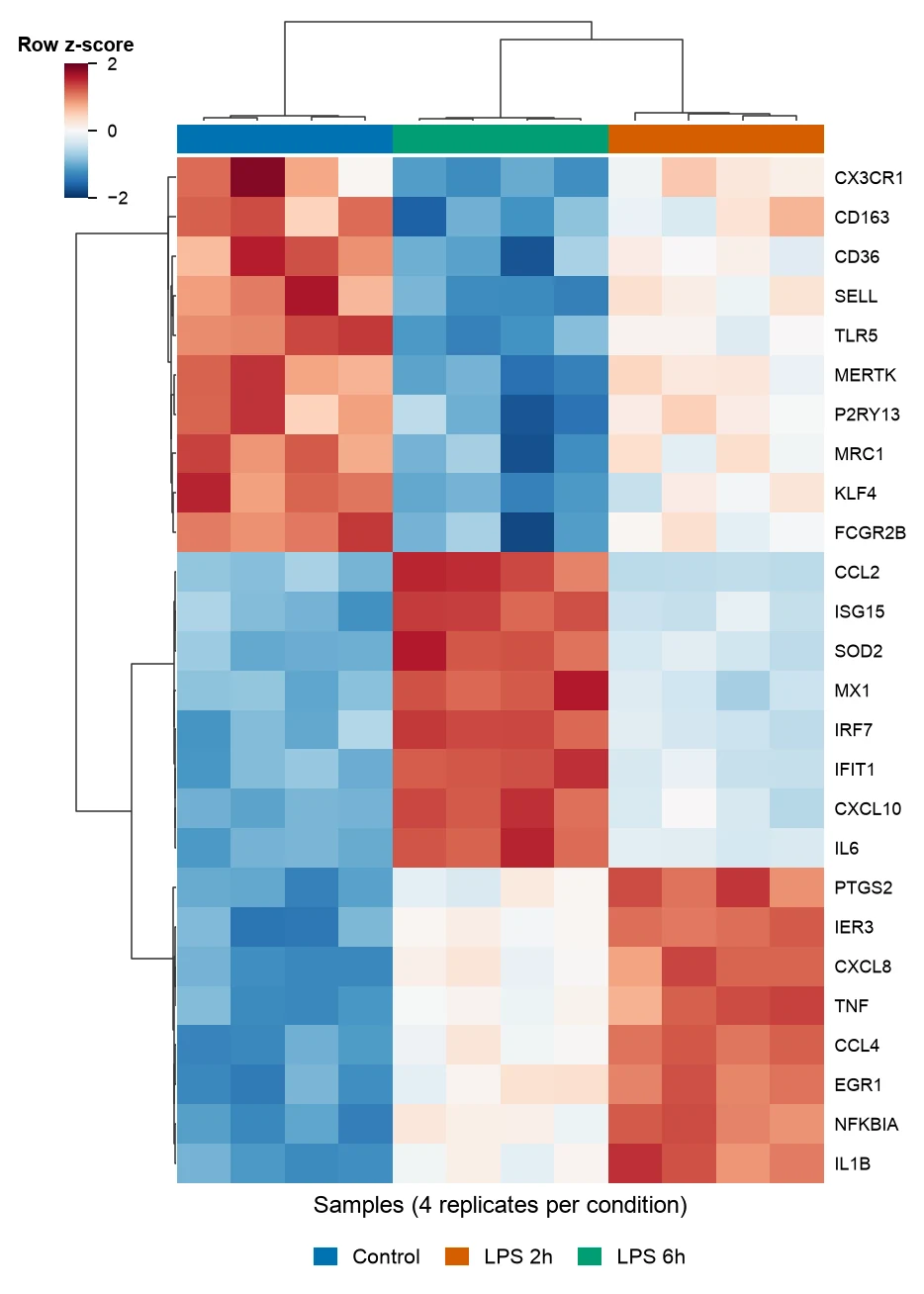
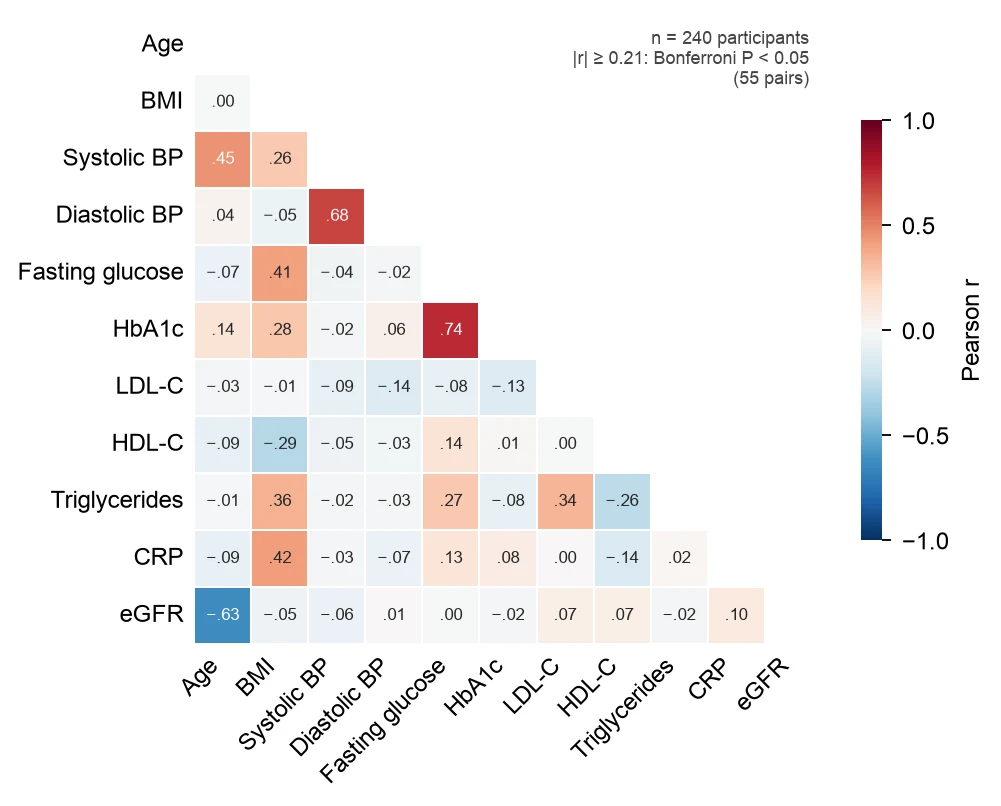
These are reference figures drawn from the sample datasets above (simulated data) to show what each prompt asks for. In the expression heatmap the 26 most variable of 32 genes fall into three clusters, genes that drop after LPS, an early response peaking at 2 h and a late interferon response at 6 h, and the 12 samples cluster by condition. In the correlation heatmap of 240 participants, 13 of the 55 pairs pass Bonferroni correction (|r| ≥ 0.21); the strongest are fasting glucose with HbA1c (r = 0.74), systolic with diastolic blood pressure (r = 0.68) and age with eGFR (r = −0.63).
What a heatmap shows
A heatmap shows a table of numbers as a grid of colored cells, so patterns across hundreds of values can be seen at once. In research the two most common kinds are the clustered gene expression heatmap, where rows are genes and columns are samples, and the correlation heatmap, where each cell is the correlation between two variables.
Gene expression heatmap with clustering
Rows are genes, columns are samples, and color is expression. Expression is usually log-transformed and then scaled per row to a z-score, so each gene is compared with its own average and a lowly expressed gene with a clear change is as visible as a highly expressed one.
Hierarchical clustering reorders rows and columns so that similar genes and similar samples sit next to each other, and the dendrograms show how they were joined. Samples that cluster by condition rather than by batch are a quick check that the experiment worked. An annotation bar above the columns shows the condition of each sample.
Correlation heatmap
A correlation heatmap shows the correlation coefficient for every pair of variables: Pearson r for roughly linear relationships, Spearman ρ for ranks or skewed data. The matrix is symmetric, so one triangle is enough, and printing r in each cell makes the figure readable without the color bar.
With k variables there are k(k − 1)/2 pairs, 55 for 11 variables, so some will look correlated by chance. Report which pairs pass a multiple-testing correction, or reorder the variables by clustering so that blocks of related measurements stand out.
Choosing a color scale
Use a diverging scale, such as blue-white-red, for values with a meaningful center: z-scores and correlations, centered at 0. Use a sequential scale such as viridis for values that only go up, such as raw expression or counts. Viridis was designed to be perceptually uniform and readable in grayscale and with color vision deficiency.
Avoid red-green scales and rainbow scales such as jet: red-green color vision deficiency affects about 8% of men of Northern European descent, and rainbow scales create sharp boundaries that are not in the data. Always show the color bar with its range.
Raw values, log scale or z-scores
Raw values let the largest numbers dominate the color range. A log2(x + 1) transform compresses counts and TPM so that fold changes become equal distances. A row z-score, (value − row mean) / row standard deviation, then puts every gene on the same scale.
Clip the scale, for example at −2 and 2, so one outlier does not wash out the rest of the figure, and say in the legend that the color is a row z-score rather than expression.
How to lay out data for a heatmap
Use a wide matrix: the first column holds row labels (genes, proteins, metabolites) and every other column holds one sample. For a correlation heatmap, use one row per subject and one numeric column per variable.
- gene
- Row label: gene symbol, protein, metabolite or any feature name. Labels should be unique.
- sample columns
- One numeric column per sample, such as log2(TPM + 1), normalized counts or intensities. Put the condition in the column name or upload a separate sample sheet.
- numeric variables
- For a correlation heatmap: one column per variable (age, BMI, glucose) and one row per subject. Non-numeric ID columns are ignored.
| gene | Control_rep1 | Control_rep2 | LPS_2h_rep1 | LPS_6h_rep1 |
|---|---|---|---|---|
| TNF | 4.73 | 5.35 | 8.49 | 6.44 |
| IL1B | 8.31 | 8.77 | 11.46 | 9.87 |
| ISG15 | 8.47 | 8.98 | 9.72 | 11.86 |
| CD163 | 6.14 | 6.69 | 6.01 | 4.92 |
Have a long table with gene, sample and value columns? Upload it as it is and ask FigCanvas to pivot it into a matrix before plotting.
How to make a heatmap with FigCanvas
Go from a data matrix to a publication-ready heatmap in four steps.
Upload a matrix or a table
Upload a CSV or Excel file with genes in rows and samples in columns, or a table of numeric variables, or load one of the sample datasets.
Confirm labels and scaling
FigCanvas identifies the row labels, the numeric matrix and any sample groups, and proposes a log transform, row z-scores, clustering or a correlation matrix.
Generate the figure
Scaling, clustering and correlations are computed from your data in Python (pandas, SciPy and seaborn are preinstalled) and drawn with journal-style defaults and colorblind-safe color scales.
Refine and export
Change the color scale, clustering, labels or annotation bars by asking in plain language, then export SVG, PDF or PNG for the manuscript.
Why researchers make their figures with FigCanvas
Clustering computed, not arranged by hand
Z-scores, distance matrices, linkage and correlation coefficients are calculated by Python code run on your data, so the order of rows and columns is reproducible.
Annotation bars and dendrograms
Sample groups appear as a color bar above the columns and the dendrograms stay aligned with the cells, the part that takes longest in pheatmap or Excel.
Colorblind-safe scales by default
Diverging blue-white-red for z-scores and correlations, viridis for raw values, with the color bar and range always shown.
Editable vector export
Export SVG or PDF and adjust fonts, gene labels or panel layout in Illustrator or Inkscape to match the journal’s figure guidelines.
Heatmap FAQs
Yes. The FigCanvas heatmap generator is made for figures in papers: upload a CSV or Excel file, say what you need in plain language, and get a clustered gene expression heatmap or a correlation heatmap. You can sign up for free and make heatmaps with the free daily credits.
Upload the expression matrix and ask for, for example, “row z-scores, cluster genes and samples, show dendrograms and a condition bar”. FigCanvas writes and runs the Python code on your data, so the clustering is computed rather than drawn by hand, and you can ask for changes in the same chat. It is the figure pheatmap(mat, scale = "row") draws in R or seaborn.clustermap in Python, without installing either.
Yes, as long as it computes from your numbers rather than drawing an image. An image generator invents the cells; FigCanvas reads your file, computes z-scores, distances and clustering in Python and colors each cell from those values, so the heatmap matches the data and can be reproduced.
A wide matrix: the first column holds row labels such as gene symbols, and each other column holds one sample, for example normalized counts or TPM exported from DESeq2 or edgeR. For a correlation heatmap, upload one row per subject and one numeric column per variable. CSV and Excel files both work, and a long table with gene, sample and value columns can be pivoted for you.
Yes; ask for it in the prompt. For expression data, apply log2(x + 1) to counts or TPM, then scale each row to a z-score, (value − row mean) / row SD, so every gene uses the same color range, and clip the scale at about ±2. Hierarchical clustering is standard: pheatmap defaults to Euclidean distance with complete linkage, while correlation distance (1 − Pearson r), used in the example above with average linkage, groups genes by the shape of their profile. Drop near-constant rows first; 6 of the 32 genes in the example were housekeeping genes with almost no variance.
Yes. Upload one column per variable and ask for Pearson r (roughly linear data) or Spearman ρ (ranks and skewed data), shown in one triangle on a diverging scale from −1 to 1 with r printed in each cell. Ask for a multiple-testing correction too: 11 variables give 55 pairs, and with Bonferroni and 240 subjects only |r| ≥ 0.21 reaches P < 0.05, as in the clinical example above.
Yes; name it in the prompt. Viridis suits sequential data and blue-white-red (ColorBrewer RdBu) suits diverging data such as z-scores; both read well with the common forms of color vision deficiency. Avoid red-green and rainbow (jet) scales: red-green color vision deficiency affects about 8% of men and 0.5% of women of Northern European descent, and rainbow scales add false boundaries.
Pro and Credit Pack users export editable SVG and 300 DPI PDF, so labels and fonts can be adjusted in Illustrator or Inkscape to the journal’s guidelines; free exports are watermarked PNG. If the journal asks for TIFF, export a PNG and convert it with the free FigCanvas PNG to TIFF converter.
It depends on where your data already lives. In R, pheatmap and ComplexHeatmap are the standard for clustered and annotated heatmaps; in Python, seaborn.clustermap. Free web tools draw heatmaps without code: Morpheus from the Broad Institute and SRplot cluster an uploaded matrix, and Heatmapper2 displays expression data, each with fixed layout options. FigCanvas takes a CSV or Excel file and a description in plain language, and returns a clustered or correlation heatmap you can export as editable SVG or PDF.
Only a simple one. Select the numbers and use Home > Conditional Formatting > Color Scales; Excel colors each cell by its value. It cannot cluster rows or columns, draw dendrograms or scale rows to z-scores, so those steps need extra formulas and manual sorting. To skip that, upload the same sheet to the FigCanvas heatmap generator.
Make a heatmap from your data
Upload an expression matrix or a table of variables, get a clustered or correlation heatmap with a colorblind-safe scale, then export it for your paper.
More AI tools for scientific figures
View all tools →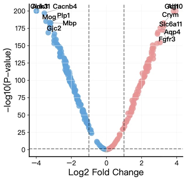
Volcano Plot Maker
Volcano plots for RNA-seq, proteomics and GWAS results with labeled genes and significance thresholds.
Open tool →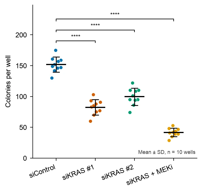
Dot Plot Generator
Dot plots that show every data point with mean or median and error bars, and bubble dot plots of marker genes across clusters.
Open tool →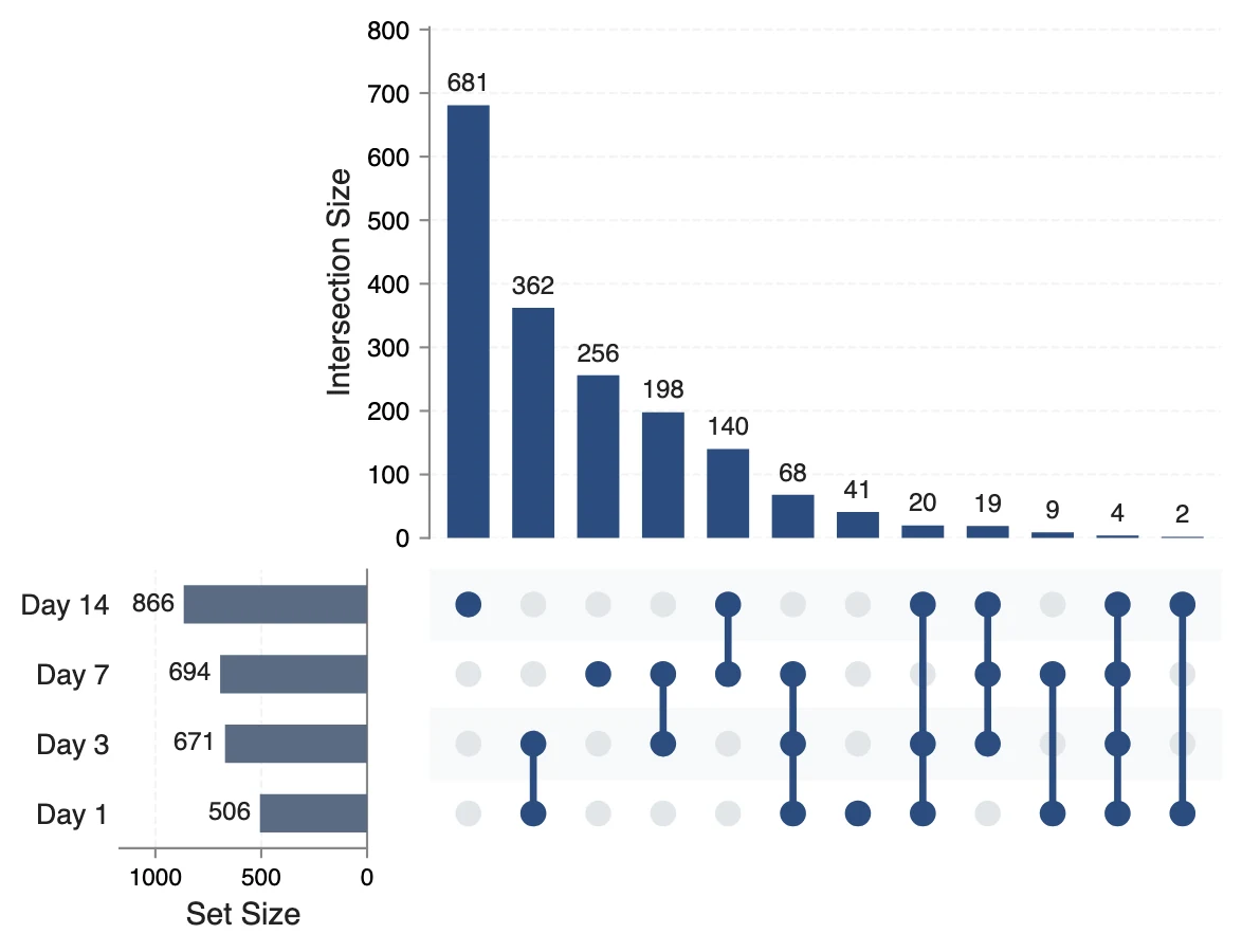
UpSet Plot Generator
UpSet plots of gene lists, variant calls or any sets, for overlaps a Venn diagram cannot show.
Open tool →